ALF snapshot and advanced play#
Recall that in the first chapter A minimal working example, we introduced
the concept of play as the process of evaluating a trained model on a task while
possibly doing some visualization. There we showed very basic usage of the
alf.bin.play module by loading a trained model and rendering the environment to
the screen or a video. Now we describe how to utilize ALF’s advanced play features
to evaluate or debug a model in depth.
ALF snapshot#
ALF calls alf.trainers.policy_trainer.play() to play a trained model. But
which code version does ALF use? By default, one expects to use the current
up-to-date code to do this. However, there are many circumstances when we don’t
want to do so. For example, we’d like to play a model that was trained a long time
ago, in one of the following scenarios:
the ALF repo is always a fixed version, but we tried out different ideas by constantly changing our own project code (e.g., algorithms) after training the model;
we wanted to use new features of ALF and pulled the lastest ALF after training the model;
as ALF developers, we updated the ALF repo constantly and it may be no longer compatible with the trained model.
These cases sound like not a big issue if we only use ALF once for all, but it does become disastrous if ALF is used for many projects repeatedly and the code version keeps evolving. Of course, version control systems like Git can help to some extent, but the key question is, how do we reliably establish a one-to-one mapping between a code version and a trained model? Git clearly is not the most satisfying answer to this.
To solve this issue, ALF uses a simple approach. Whenever lauching a training
(alf.bin.train) or grid searching (alf.bin.grid_search) job, ALF
takes a snapshot of the current repo and stores it in the job root dir. For example,
the following command
python -m alf.bin.train --root_dir /tmp/alf_tutorial1 --conf <ALF_ROOT>/alf/examples/tutorial/minimal_example_conf.py
will store an ALF snapshot at /tmp/alf_tutorial1/alf. The snapshot directory
has exactly the same structure with the ALF repo (i.e., it is a clone).
Note
ALF relies on rsync
to copy all *.py, *.gin, and *.json files of the ALF repo to
a snapshot. The size of a snapshot is roughly 15M which is acceptable given
modern disk storage capacity.
In this way, each trained model is accompanied with an ALF snapshot which is exactly the code version that trained that model. Even if we implement our own algorithms without touching ALF, our own code will get a snapshot if its path starts with the ALF root.
Note that in the case of continuing training an existing root_dir, a new snapshot
will be generated to overwrite the existing one.
python -m alf.bin.train --root_dir /tmp/alf_tutorial1
This will generate a new snapshot at /tmp/alf_tutorial1/alf.
When playing a trained model with snapshot enabled, we can add an option --use_alf_snapshot
to use the archived ALF version instead of the current one:
python -m alf.bin.play --root_dir /tmp/alf_tutorial1 --use_alf_snapshot
You’ll notice some message like
I0914 11:49:21.344848 140367115069248 play.py:168] === Using an ALF snapshot at '/tmp/alf_tutorial1/alf' ===
which indicates that you’re indeed using a snapshot version.
Note
It’s possible to turn off the snapshot feature. When training or grid searching,
appending the option --nostore_snapshot will do so.
The special case of config file#
The config file of a training job will also be archived in a snapshot, if its
path starts with ALF root. However, ALF also archives another config copy
directly under the job directory named as alf_config.py. This special config
file also records command-line config parameters and grid search parameters, so
it’s generally more accurate than the snapshot version.
In the above training example, if we add a command-line config parameter:
rm -rf /tmp/alf_tutorial1
python -m alf.bin.train --root_dir /tmp/alf_tutorial1 --conf <ALF_ROOT>/alf/examples/tutorial/minimal_example_conf.py --conf_param="TrainerConfig.summary_interval=100"
Again, ALF will store a snapshot at /tmp/alf_tutorial1/alf and we can get
the config file at
/tmp/alf_tutorial1/alf/examples/tutorial/minimal_example_conf.py
However, this is just a copy of the original config file: it doesn’t record
our command-line parameter TrainerConfig.summary_interval=100.
In contrast, if we look at /tmp/alf_tutorial1/alf_config.py, we’ll see something
like
########### pre-configs ###########

import alf
alf.pre_config({
    'TrainerConfig.summary_interval': 100,
})

########### end pre-configs ###########
on the very top of the file.
Regardless of whether having the flag --use_alf_snapshot when playing a model,
ALF will always use alf_config.py. So if we’d like to make changes to the
config file for play, we need to modify alf_config.py in either case.
For other changes to make for play, we need to modify the snapshot code if
--use_alf_snapshot is provided, and modify the current ALF repo otherwise.
Advanced play by rendering#
Besides playing with a snapshot, another advanced play case is to utilize the
alf.summary.render module. This module contains several helper functions
that convert arrays and tensors to Image objects for visualization
on screen or in a video. Recall that ALF’s play calls an algorithm’s
predict_step() to do online action prediction given
a trained model (see algorithm interfaces). The AlgStep
output of a predict_step() call will be used for environment interaction and
retrieve the next environment frame. At every step of this prediction loop, any
Image object, once put into info of an AlgStep returned
by an algorithm’s predict_step(), will be concatenated to the corresponding
environment frame by the side. Below we’ll walk through an example to show how to
use alf.summary.render. The complete code is located at alf.examples.tutorial.ac_render_conf.
We will again train a model on the “CartPole-v0” task. So first of all, we activate
all the configurations of alf.examples.ac_cart_pole_conf by importing it:
from alf.examples import ac_cart_pole_conf
And import the render module
import alf.summary.render as render
Then to tell the play module what to render, we overwrite
predict_step() of the original AC algorithm:
class ACRenderAlgorithm(ActorCriticAlgorithm):
   def predict_step(self, inputs, state):
       alg_step = super().predict_step(inputs, state)
       action = alg_step.output
       action_dist = alg_step.info.action_distribution
       with alf.summary.scope("ACRender"):
           # Render an action image of type ``render.Image``.
           action_img = render.render_action(
               name="predicted_action",
               action=action,
               action_spec=self._action_spec)
           # Render an action distribution image of type ``render.Image``.
           action_dist_img = render.render_action_distribution(
               name="predicted_action_distribution",
               act_dist=action_dist,
               action_spec=self._action_spec)
       # Put the two ``Image`` objects into ``info``. Any nest structure is
       # acceptable for the new ``info``. ALF's play will look for ``Image``
       # objects.
       return alg_step._replace(
           info=dict(action_img=action_img,
                     action_dist_img=action_dist_img,
                     ac=alg_step.info))
Basically, what we’d like to do is taking the predicted action and action distribution
from the AlgStep of ActorCriticAlgorithm, and call render.render_action()
and render.render_action_distribution() to obtain two Image
objects. The final step is to make sure to put the objects in the info field of
the returned AlgStep. It doesn’t matter how we organize the two objects in info:
as long as they are in it, play will find and display them.
Note that we created a namescope of “ACRender” when calling the rendering functions. This namescope usage is exactly the same with the namescope for summary functions: it will prefix all rendered image names with “ACRender/”. These image names will be displayed as labels in the final video.
Finally, we tell ALF to use our newly defined algorithm:
alf.config(
    "TrainerConfig",
    algorithm_ctor=partial(
        ACRenderAlgorithm, optimizer=alf.optimizers.Adam(lr=1e-3)))
Now let’s train and play this conf file:
python -m alf.bin.train --root_dir /tmp/ac_render --conf <ALF_ROOT>/alf/examples/tutorial/ac_render_conf.py
# After several minutes the above training command will finish.
# Once finished, Run the following command to play the trained model.
python -m alf.bin.play --root_dir /tmp/ac_render --num_episodes 1 --record_file /tmp/tmp.mp4 --alg_render
Note that when playing, we need to add the flag --alg_render to turn on the
render module; otherwise the rendering functions will not
be called. If we open “tmp.mp4”, the video frame will look like:

Basically, along with every environment frame, the action taken at that frame will also be displayed.
render contains other rendering functions (e.g., heatmap,
curve, etc), and we suggest the reader to take a look at its API doc. Some example
rendered frames are:


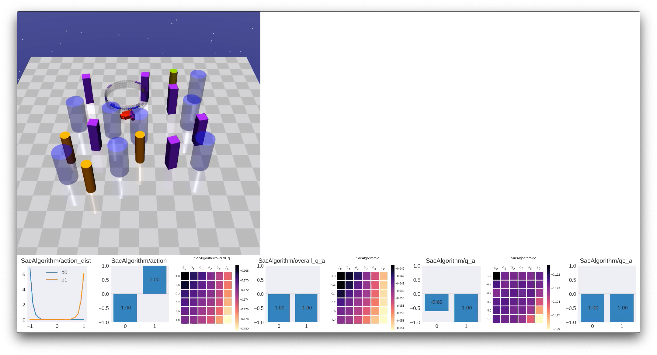
Note
Currently with --alg_render the rendering speed will be slow (less than
10 FPS, depending on how many plots each frame has). This
inefficiency is largely due to Matplotlib.
Summary#
In this chapter we explained what ALF snapshot is, why we need it, and how to use it for playing a model. We also talked about how to customize rendering during play to visualize various prediction statistics. These two advanced play use cases enable us to better evaluate and analyze trained models.